Transformer Recommenders: Designing the Training and Serving Systems

Alok Upadhyay | April 2026 · Explainer

TL;DR: The modelling shift in recommenders, from “score a user–item pair” to “predict the next action in a sequence”, is well documented. The systems shift that comes with it is less so, and it is where most of the value is won or lost. Two properties decide the outcome: whether your training examples could have seen the future, and whether the features at serving time are produced by the same code that produced them at training time.

What actually changed

Classical recommenders factor a user–item interaction matrix, or run a two-tower model that embeds user and item separately and takes a dot product. The user is a vector: a summary, order discarded.

Sequential transformers drop that summary. The input becomes the user’s action history in order, and the task becomes next-action prediction. SASRec (Kang and McAuley) established the causal self-attention formulation; BERT4Rec (Sun et al.) explored the masked variant. More recent work pushes further: generative retrieval assigns each item a short code, a semantic id, and decodes ids directly rather than searching an embedding space (Rajput et al. on TIGER), and scaling work like HSTU (Zhai et al.) treats the whole thing as a sequence-transduction problem large enough to show language-model-like scaling behaviour.

The practical consequence is what matters here. The model’s input is no longer a precomputed user vector you can refresh nightly. It is a sequence that changes every time the user does anything. That single fact drives nearly every system decision below.

The training system

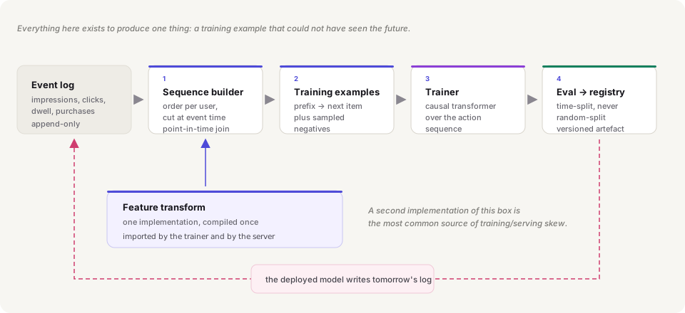Training pipeline for a sequential recommender: event log, point-in-time sequence builder, training examples, trainer, evaluation and registry, with a shared feature transform and the feedback loop back into the log Everything in the pipeline exists to produce one thing: a training example that could not have seen the future.

Point-in-time correctness is the whole job

For a given user at a given moment, a training example must contain exactly what was knowable then. This sounds obvious and is violated constantly, because the natural way to build features is to join against current tables, and current tables contain the future.

The failure is seductive rather than loud. Offline metrics improve. The model has learned to use information that will not exist at serving time, so online performance does not move, or moves down. A sequence model is more exposed than a two-tower model here, because it consumes many timestamped events per example rather than one aggregate, and each is a chance to leak.

Concretely, the things that leak most often:

Aggregates computed over the full table: an item’s lifetime popularity includes clicks that happen after the example’s timestamp
Slowly-changing dimensions read as current: a user’s country or subscription tier as of today, not as of the event
Label windows that overlap the feature window: a seven-day conversion label with features computed through day seven
Deduplication after the cut: dropping events “already seen” using knowledge that arrived later

The defence is structural, not procedural: the sequence builder takes an as-of timestamp, and every join is a temporal join against that timestamp. Once any feature can be computed without one, leakage is a matter of time.

Split by time, never at random

A random split lets the model train on Friday and test on Wednesday. Reported accuracy is then partly a measure of how well it interpolates within a period it has already seen, which is not the question. Split by time, and keep a gap between train and eval that matches your real deployment lag.

Negatives are a modelling decision disguised as a data decision

Next-item prediction over a catalogue of 10⁸ makes a full softmax impractical, so you sample. The sampling scheme is not an implementation detail:

In-batch negatives are cheap and biased toward popular items, because popular items appear in batches more often. Uncorrected, the model learns that popular things are good, which it will then recommend, making them more popular.
Sampled softmax with a log-Q correction removes much of that bias and is usually worth the complexity.
Hard negatives, items retrieved but not engaged with, teach the boundary that matters, and are what the ranking stage actually faces in production.

Popularity bias here compounds through the feedback loop drawn at the bottom of the diagram. The model’s outputs become tomorrow’s training data. A mild popularity skew, retrained on its own recommendations, is not stable; it tightens.

One feature transform, imported twice

If the trainer and the server each have their own implementation of feature construction, they will diverge. Not in principle; in practice, within a quarter, and silently. One implementation, compiled once, imported by both paths. Then a skew test that asserts equality on live traffic, because “we share the code” degrades into “we shared the code in March.”

The serving system

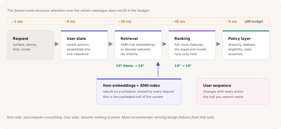Serving path: request, user state assembly, candidate retrieval, ranking and policy layer, with a latency budget and the caches each stage depends on Item side: precompute everything. User side: assume nothing is warm. Most of the serving design follows from that split.

The funnel exists because attention does not scale to the catalogue

You cannot run a cross-attention model over 10⁸ items inside a 75 ms budget. So the work is staged: cheap retrieval narrows 10⁸ to ~10³, expensive ranking narrows 10³ to ~10¹.

Retrieval has two shapes now. The established one embeds the user sequence into a vector and runs approximate nearest neighbour against precomputed item embeddings: fast, well understood, and the index is shared across all requests. The generative alternative decodes semantic ids directly with beam search, which removes the ANN index entirely and lets the model express item structure in the code itself. It also puts autoregressive decoding on the critical path, which is a real latency cost and a real operational change. Worth understanding; not automatically worth adopting.

Ranking is where the expensive model belongs. With only ~10³ candidates you can afford full cross-features between the user sequence and each item.

What is cacheable, and what never is

This is the split that organises everything:

Item embeddings and the ANN index are shared across all users and rebuilt on a schedule. Precompute aggressively.
The user sequence changes with every action. A cache keyed on user id is stale precisely when it matters most: the user just did something, which is usually why they are being served again.

Which means the sequence encoder sits on the critical path for every request. The usual mitigations are to cap sequence length at the point where marginal events stop paying for themselves, and to cache the encoding of the stable prefix while recomputing only the recent tail.

Budget the latency explicitly

The numbers on the diagram are illustrative, but the discipline is not: assign each stage a p99 budget and enforce it. Recommender latency failures are rarely one slow component; they are four stages each 30% over, discovered together during a traffic peak.

Training/serving skew, concretely

Skew is the gap between what the model saw in training and what it sees in production. Common sources, in rough order of how often they bite:

Source	How it shows up
Two feature implementations	Offline gain fails to replicate online
Sequence truncated differently	Long-history users degrade first
Different tokenisation of ids	New or rare items behave erratically
Serving-time fallbacks on missing data	Silent quality loss for a user segment
Log sampling before training	Model trained on a biased slice of traffic

The one worth calling out is the fourth. Serving code frequently substitutes a default when a feature is unavailable. Training data, drawn from complete logs, rarely contains that default. The model has never seen the value it is now being given, and its behaviour on it is undefined, for whichever users happen to trip that path.

What to watch

offline/online delta   the gap between predicted and realised gain,
                       tracked per launch, not per quarter

skew test              assert train and serve features match on a
                       sample of live traffic, continuously

sequence length        p50 and p99 of history actually used
                       vs. the cap you set

catalogue coverage     share of the catalogue appearing in any slate;
                       the feedback loop shows up here first

stage latency          p99 per stage against its budget, not end to end

Catalogue coverage is the early-warning signal. Engagement metrics can look healthy while the system quietly collapses onto a shrinking set of items, the feedback loop tightening. By the time it registers in engagement, several retraining cycles have baked it in.

The one-sentence version

The modelling change is the easy half; the systems change is making sure every training example is a faithful snapshot of a moment, and that production reconstructs that snapshot with the same code. Everything else is a funnel built to fit a latency budget.