RLHF Post-Training: Designing the Training and Serving Systems

Alok Upadhyay | July 2026 · Explainer

TL;DR: The RLHF objective fits on one line. The system it implies does not. PPO-style RLHF is the only common training job that holds four copies of a model in memory at once and runs a sampler and a trainer inside the same process group, and the thing that actually reaches production is one of those four, selected by a judge that was deliberately kept out of the optimisation. Most of the engineering difficulty lives in those two sentences.

---

The objective, only as far as we need it

Three stages, briefly, because every system decision below is downstream of them.

Supervised fine-tuning takes a pretrained base model and fine-tunes it on demonstrations. Ordinary cross-entropy. What it produces is less a finished model than a starting position: format, register and refusal behaviour fixed well enough that sampling from it yields usable candidates.

The reward model is trained on pairwise comparisons, not absolute ratings, typically under a Bradley–Terry likelihood:

$$\mathcal{L}_{\text{RM}} = -\log \sigma\big(r(x, y_w) - r(x, y_l)\big)$$

Only the difference between scores is constrained. The absolute scale is unidentified: add a constant to every reward and the loss is unchanged. A reward model’s output is meaningful as an ordering and close to meaningless as a magnitude, which is worth remembering before you build a dashboard around raw reward values.

The policy update maximises that reward under a penalty for moving:

$$\max_{\pi}\; \mathbb{E}_{y \sim \pi(\cdot \mid x)}\big[\, r(x, y) \,\big] \;-\; \beta\, \mathrm{KL}\big(\pi(\cdot \mid x)\,\|\,\pi_0(\cdot \mid x)\big)$$

The constraint is not a regulariser bolted on for stability; it is the method. The reward model is trustworthy near the distribution it was trained on and unreliable away from it, so the KL term keeps optimisation inside the region where the proxy still means something.

Now read that objective as an infrastructure specification. It says: hold π and π₀ at the same time, because you need log-probabilities from both on the same tokens. It says: hold r, because you need to score samples. It says y ∼ π, which means you must generate before you can learn. The training data does not exist until the model makes it. Everything below follows from those three demands.

The training system

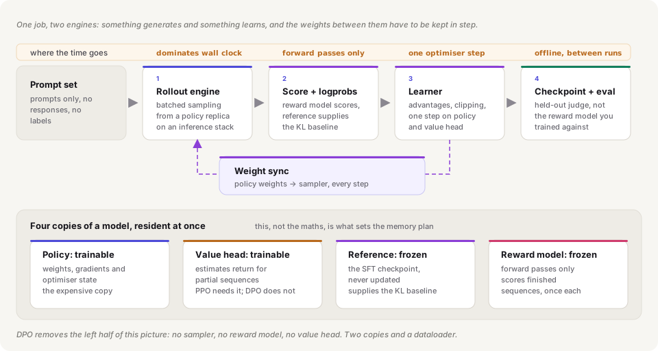One job, two engines: something generates and something learns, and the weights between them have to be kept in step.

Four model copies, and that is the memory plan

Most training jobs hold one model. A PPO-style RLHF job holds four, and they are not interchangeable:

• Policy: trainable. Carries weights, gradients and optimiser state. If you are on a sharded optimiser this is the copy whose footprint is several times its parameter count.
• Value head / critic: trainable. Estimates expected return for partial sequences so advantages are not pure Monte Carlo. Often a small head on a shared trunk, sometimes a full second model; that choice alone can swing the memory budget.
• Reference: frozen. The SFT checkpoint, forward passes only, used solely to produce log π₀(y|x) for the KL term.
• Reward model: frozen. Forward passes only, one score per finished sequence.

Two of those carry gradients and two do not, and that asymmetry is the main lever. The frozen copies need no optimiser state, no gradient buffers and no activation retention, so they can be quantised harder, sharded differently, or moved off the training devices entirely and called as a service. The temptation to “just put everything on the same devices” is what produces an out-of-memory error two hours into a run, at exactly the point where sequence lengths grow because the policy has learned to write longer answers.

A few placement decisions worth making deliberately rather than by default:

• Reward model as a separate service. It is stateless, frozen, and called once per completed sequence. It behaves like an inference workload, so run it like one: its own replicas, its own batching, its own scaling. The cost is a network hop inside the loop; the benefit is that it stops competing for memory with the thing that needs it.
• Reference model co-located with the policy. This one is harder to externalise, because it needs per-token log-probabilities over the same token ids the policy just produced, and shipping those tensors around is not free. Co-locating it and accepting the memory is usually right.
• Shared trunk for the value head. Cheap in memory, and it couples the critic’s representation to the policy’s, which is fine while the policy is near the reference and less fine once it has moved.

Two engines in one job

The distinctive shape of PPO-style RLHF is that it needs an inference system and a training system running inside the same job, alternating.

Generation wants large batches, KV caching, continuous batching, paged attention, low-precision weights, everything a serving stack is built around. The gradient step wants sharded optimiser state, activation checkpointing, high-precision accumulation, collective communication. These are different engines with different memory layouts, and in practice you end up with two of them: a generation runtime holding a replica of the policy, and a training runtime holding the authoritative copy.

Which creates the thing that is genuinely specific to this workload.

Weight synchronisation is the coupling

After every optimiser step, the sampler’s copy of the policy is stale. If you keep sampling from it, you are doing off-policy updates with a ratio that PPO’s clipping was not designed to absorb, and the run degrades in ways that look like a hyperparameter problem and are not.

So the weights have to move: trainer → sampler, on a cadence you choose. This is a real cost, and it scales with model size rather than with batch size, so it gets relatively worse as the model gets bigger. The usual designs:

• Collective broadcast into co-located sampler ranks. Fastest when the two engines share hosts, and the reason many RLHF frameworks insist on co-location even though it complicates scheduling.
• Checkpoint round-trip through shared storage. Simple, debuggable, and slow enough that you will find yourself syncing every N steps instead of every step, which reintroduces the staleness you were avoiding.
• Partial or delayed sync, accepting bounded off-policyness deliberately and correcting for it in the objective rather than pretending it is not there.

The honest framing is that sync cadence is a throughput/correctness dial, not a detail. Tighten it and you spend wall clock moving tensors; loosen it and you spend it on a policy drifting away from the distribution its updates assume.

Rollout generation is the bottleneck

The instinct from ordinary training is that the backward pass dominates. In RLHF it usually does not. A single optimiser step consumes a batch of rollouts, and producing those rollouts means autoregressive decoding: sequential, memory-bandwidth-bound, and as long as the responses you want to train on. The forward passes for reward and reference are a single pass each over a completed sequence; the gradient step is one pass over the batch. Generation is hundreds of sequential steps per sample.

The consequences are all scheduling consequences:

• Rollout length is a budget item. Longer maximum response lengths cost generation time superlinearly once KV cache pressure forces smaller batches. And the policy tends to grow its responses during training, so the budget you set on day one is not the budget you are spending on day three.
• Stragglers set the pace. A batch finishes when its slowest sequence finishes. Length-bucketing prompts, capping generation, and allowing partial batches all help; naive synchronous batching wastes a large fraction of the sampler.
• The trainer idles while the sampler works, unless you overlap them. Generating the next batch of rollouts while the current one is being learned from is the standard fix, and it is also a deliberate decision to be one step off-policy.
• Scale the two sides independently. If generation is the wall, more sampler replicas help and more trainer ranks do not. Treating the job as one homogeneous pool hides that.

Checkpointing, and what to keep

Checkpoint on a KL schedule, not only on a step schedule. The interesting artefacts are the policies at a few different distances from the reference, because, as the next section argues, you cannot know in advance which distance is the right one, and you will want candidates to choose between. Log reward and KL alongside each checkpoint so the selection stage has something to work with.

Why DPO’s system profile is radically simpler

Direct Preference Optimization (Rafailov et al.) starts from the observation that the constrained objective has a closed-form optimum expressible in terms of policy and reference log-probabilities. Rearranged, the reward model disappears as a separate artefact and you fine-tune directly on preference pairs with a classification-style loss.

As a system, that deletes most of the left half of the diagram:

	PPO-style	DPO-style
Model copies resident	four	two
Sampling loop in the job	yes	no
Reward model at train time	hosted and called per rollout	not present
Weight synchronisation	required	not applicable
Data	generated on the fly	a fixed dataset
Shape of the job	RL system	supervised fine-tuning

That last row is the point. DPO is an ordinary dataloader-plus-trainer job with one extra frozen forward pass, which means it runs on infrastructure you already have and fails in ways you already understand.

What it does not remove is the constraint. The reference model and β are still there, doing the same job. And it trades one problem for another: PPO samples from the current policy, so the reward model sees the policy’s own mistakes as they develop, while DPO optimises against a fixed dataset collected from some earlier distribution. As the policy moves, that data describes it less and less well. Neither is strictly better. They fail differently, and which failure you prefer depends on how much you trust your preference data relative to your reward model.

The serving system

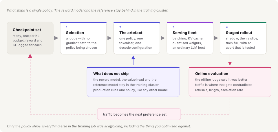Only the policy ships. Everything else in the training job was scaffolding, including the thing you optimised against.

The artefact is smaller than the job

This is worth stating plainly because diagrams of RLHF rarely do: the reward model and the reference model do not go to production. Neither does the value head. What ships is one policy, one tokeniser, and a decode configuration: the same artefact shape as any other fine-tuned language model. There is no KL term at inference time. There is no reward being computed. The constraint did its work during training and left no trace in the serving path except the weights it shaped.

Which means the serving system for an RLHF-tuned model is, mechanically, an ordinary LLM serving system: continuous batching, KV cache management, quantised weights, a latency budget split between time-to-first-token and inter-token latency. That part is not special and this post will not pretend otherwise.

What is special is everything around the decision to ship, and the fact that the model’s most distinctive property, that it was optimised against a proxy, is invisible from inside the serving stack.

Selection is the load-bearing step

Reward over-optimisation has a characteristic shape, and it has been studied directly; Gao, Schulman and Hilton’s work on scaling laws for reward-model over-optimisation is the standard reference. Proxy reward increases monotonically. True quality, measured by a held-out judge the policy is not being trained against, rises, peaks, and then falls. The peak is not at convergence. Training to convergence on the proxy is training past the point of usefulness.

The systems consequence is a hard constraint on the selection stage: you cannot select a checkpoint using the reward model you trained against. It is the quantity being exploited; asking it which checkpoint is best is asking the proxy to grade its own exploitation. You need an evaluator with no gradient path to the policy:

• a held-out judge model that was never used to produce training signal, ideally from a different lineage
• a separate rater pool scoring blind pairwise comparisons against the reference
• a task-grounded metric: unit tests that pass, an answer that matches ground truth, a tool call that executes, none of which can be talked into a higher score

Design the pipeline so this separation is structural rather than a matter of discipline. The reward model artefact and the judge artefact should be different registry entries with different provenance, and the selection job should not have credentials to load the reward model at all. “We were careful about which model we used” degrades into “we were careful in March.”

The output of selection is not a single number either. A rising reward curve on its own tells you almost nothing; reward rising at an acceptable KL is the claim worth making. Report reward and KL together, and pick from the candidates on the frontier rather than the one with the highest proxy score.

Guardrails around a freshly-tuned policy

A newly RLHF’d policy is the least-tested component in the stack. It was shaped by an optimiser that was, by construction, searching for whatever scored well, including things nobody intended to reward. The guardrails that matter are the ones that assume the model has learned something surprising:

• Decode configuration is part of the artefact. The policy was trained under a particular sampling regime. Serving it at a very different temperature or with different penalties is a distribution shift the KL constraint never saw. Pin it with the weights and version it with the weights.
• Length and repetition limits. Length inflation is the most common RLHF artefact, and it shows up first as a latency and cost regression, not as a quality one.
• Safety filters stay independent of the policy. If the same preference data that tuned the policy also tuned the filter, they share failure modes and the filter will nod along with exactly the outputs it should catch.
• A tested abort path. Not a rollback plan on a wiki, but a traffic switch someone has actually exercised, because the quality failures RLHF produces are fluent and confident and will not trip an error rate alarm.

Staged rollout, because offline evaluation is a proxy too

The judge that selected the checkpoint is itself a model of what people want. It is a better proxy than the reward model, and it is still a proxy. So: shadow traffic first (generate, log, do not serve), then a small slice, then wider, with the online comparison being against the current production policy, not against the reference the training job used.

The signals worth carrying through staging are the ones the training objective could not see: refusal rate on benign requests separately from harmful ones, response length as a distribution, escalation and retry rates, and whatever task-grounded success metric the surface actually has. Aggregate quality scores move slowly and hide the trade you care about.

The loop back to preference collection

Production traffic is where the next round of preference data comes from, and this is the point where the serving system feeds the training system.

There is a subtlety that bites reliably. Preference pairs are collected from the outputs of some policy. Once you ship the tuned model, that policy no longer exists: the data you are collecting describes the new one, and the data you collected last quarter describes a model you have replaced. Training the next round on stale pairs optimises against a distribution nobody is serving.

So the collection pipeline should record which policy version produced each response, and the training pipeline should be able to filter on it. This sounds like metadata hygiene and is actually the difference between a preference dataset that compounds and one that quietly describes the past.

Failure modes, systems flavour

Failure	What you observe	Usual cause
Out of memory mid-run	Job dies well after it started, often as responses lengthen	Four model copies co-located; no headroom for growing KV cache
Sampler/trainer imbalance	Devices idle, throughput far below either engine alone	Synchronous rollouts, no overlap, stragglers setting the pace
Stale reference or sampler weights	Training destabilises; looks like a hyperparameter problem	Sync cadence loosened for throughput, or reference accidentally updated
Reward model drift	Reward rises smoothly, blind evaluations do not	Policy has moved off the distribution the reward model was fit on
Checkpoint selected on the proxy	Offline gain fails to replicate online	Selection used the reward model, or a judge sharing its training data
Stale preference data	Each round helps less than the last	Pairs collected from a policy that is no longer being served
Length inflation	Latency and cost regress before quality does	Raters mildly preferred longer text; nothing in the loop penalised it
Sycophancy	Model agrees with incorrect user claims	Agreement was rewarded during ranking

None of these are bugs in the algorithm. The first three are the optimiser and the scheduler disagreeing about what the job is; the rest are the optimiser doing exactly what it was asked, against an objective that encoded something slightly different from what was meant.

What to instrument

reward               rising, but read only alongside KL, never alone

KL(pi || pi_0)       the budget actually being spent; the x-axis of
                     every checkpoint decision

rollout throughput   sequences/sec from the sampler, and the fraction
                     of wall clock the trainer spends idle

sync latency         time to move weights trainer -> sampler, and the
                     step lag between them

response length      per response, as a distribution not a mean, on
                     both the training rollouts and production traffic

win-rate             vs. the reference, judged by an evaluator with
                     no gradient path to the policy

refusal rate         on a benign set and a genuinely harmful set,
                     reported separately

policy version       stamped on every logged response, so preference
                     data can be filtered by the model that produced it

Two of these earn their place by being unusual. Trainer idle fraction is the fastest way to discover that your RLHF job is a generation job wearing a trainer’s clothes; if it is high, no amount of gradient-side optimisation will help. And refusal rate split in two hides nothing: a single aggregate number conceals the trade you actually care about, which is refusing more of what should be refused without refusing more of what should not.

---

The one-sentence version

RLHF’s objective asks you to hold four models at once and to generate your own training data, which makes the training job a sampler and a trainer fighting over the same devices with weights shuttling between them, and then ships exactly one of those models, chosen by a judge you were careful to keep out of the optimisation, because the thing you optimised against is the last thing you should trust to tell you when to stop.